Implementing Pivot Reversal Strategy in Python with vectorbt

The pivot reversal strategy is a popular trading strategy for crypto. It is based on the principle of buying or selling when the price of an asset hits a certain level, signaling a possible reversal in its trend. This strategy can be used to capitalize on short-term price movements in crypto markets. So I decided to implement it in Python with the help of vectorbt framework.

First let’s import libraries needed in our development:

import pandas as pd
import vectorbt as vbt
import numpy as np
import datetime

Next, we need to load data. I’m loading data from my data warehouse, but you can use any other data source. In my blog, I have many articles with examples of how to load bars from Binance, ByBit, and EOD for stocks for example. For his example, I’m using 1h data for ETHUSDT from 2020:

data_hist = pd.read_parquet("/data/binance/spot/1h/ETHUSDT.parquet")
data = data_hist[data_hist.index > datetime.datetime(2020, 1, 1)].copy()

Next, I’ll specify the parameters needed for Pivot Points. I need to set only left, and right bars, and also I’m using min tick because I’m using it in setting stop/limit orders.

left_bars = 5
right_bars = 5
min_tick = 0.0001

Next, let’s do the needed computations. For simplicity and speed, I’m doing everything in numpy and pandas. Next, let’s compute our pivot points. In total, we’ll have 4 variables:

shw_cond – true/false where swing high is happening
shl_cond – true/false where swing high is happening
hprice – last swing high price
lprice – last swing low price

Calculations are pretty simple. We just compare the highs/lows of the current bar with the needed amount of highs/lows around it.

# Swing High, Condition and hprice
data["swh_cond"] = (data.high >= data.high.rolling(left_bars).max().shift(1)) & \
                   (data.high >= data.high.rolling(right_bars).max().shift(-right_bars))
    
data["hprice"] = np.where(data['swh_cond'], data.high, np.nan)
data["hprice"] = data["hprice"].fillna(method='ffill').shift(right_bars).fillna(value=0)

# Swing Low, Condition and lprice
data["swl_cond"] = (data.low <= data.low.rolling(left_bars).min().shift(1)) & \
                   (data.low <= data.low.rolling(right_bars).min().shift(-right_bars))

data["lprice"] = np.where(data['swl_cond'], data.low, np.nan)
data["lprice"] = data["lprice"].fillna(method='ffill').shift(right_bars).fillna(value=0)

Next, let’s compute signals themselves as crossovers of high/low and recent pivot high/low levels:

# Long crossover
data["Long entries"] = (data.high >= data.hprice.shift(1) + min_tick) & (data.high.shift(1) < data.hprice.shift(2) + min_tick)

# Short crossover
data["Short entries"] = (data.low <= data.lprice.shift(1) - min_tick) & (data.low.shift(1) > data.lprice.shift(2) - min_tick)

In vectorbt we’ll simulate stop orders, so we need to save the price at wich I want to execute my orders. We’ll create a separate column for it:

data["trade_price"] = np.where(data["Long entries"], \
                               data.hprice + min_tick, \
                               np.where(data["Short entries"],data.lprice - min_tick, np.nan))

Now we have everything ready to calculate our strategy using vectorbt engine:

pf = vbt.Portfolio.from_signals(
  data.close,
  entries=data["Long entries"],
  short_entries=data["Short entries"],
  upon_opposite_entry="ReverseReduce",
  price=data["trade_price"],
  freq='1h'
)

Out backtest is computed, so now we can output some statistics. stats() method will output the main metrics for our strategy:

pf.stats()

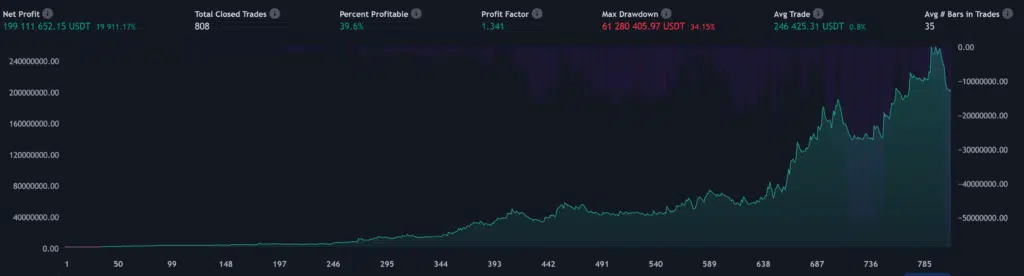
Start                               2020-01-01 01:00:00
End                                 2023-02-06 23:00:00
Period                               1131 days 16:00:00
Start Value                                       100.0
End Value                                  24143.734197
Total Return [%]                           24043.734197
Benchmark Return [%]                          1135.6782
Max Gross Exposure [%]                            100.0
Total Fees Paid                                     0.0
Max Drawdown [%]                              37.005134
Max Drawdown Duration                 136 days 17:00:00
Total Trades                                        809
Total Closed Trades                                 808
Total Open Trades                                     1
Open Trade PnL                                82.733924
Win Rate [%]                                  39.727723
Best Trade [%]                                56.521998
Worst Trade [%]                              -12.492299
Avg Winning Trade [%]                          5.626995
Avg Losing Trade [%]                            -2.3353
Avg Winning Trade Duration    2 days 05:04:51.588785046
Avg Losing Trade Duration     0 days 20:44:06.406570841
Profit Factor                                  1.422016
Expectancy                                    29.654703
Sharpe Ratio                                   2.460286
Calmar Ratio                                  13.156512
Omega Ratio                                    1.083777
Sortino Ratio                                  3.658924

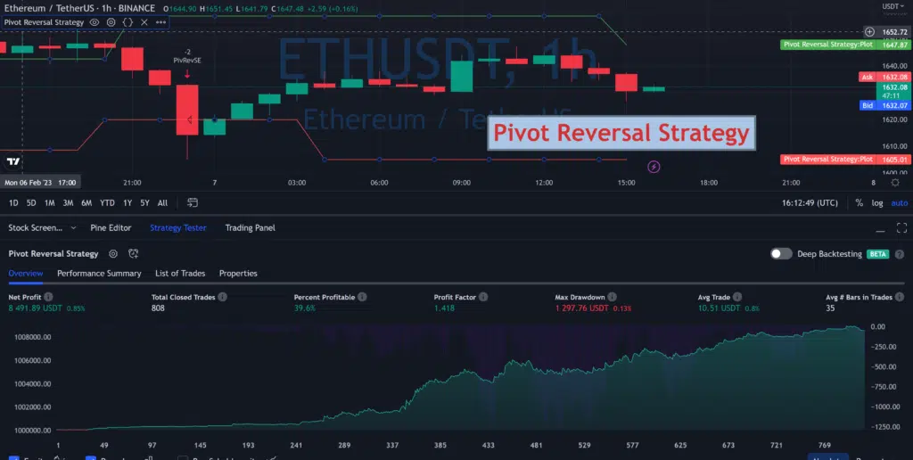
If we’ll compare this with the output of PineScript for the same period/instrument/timeframe, we’ll see that we’re quite close: