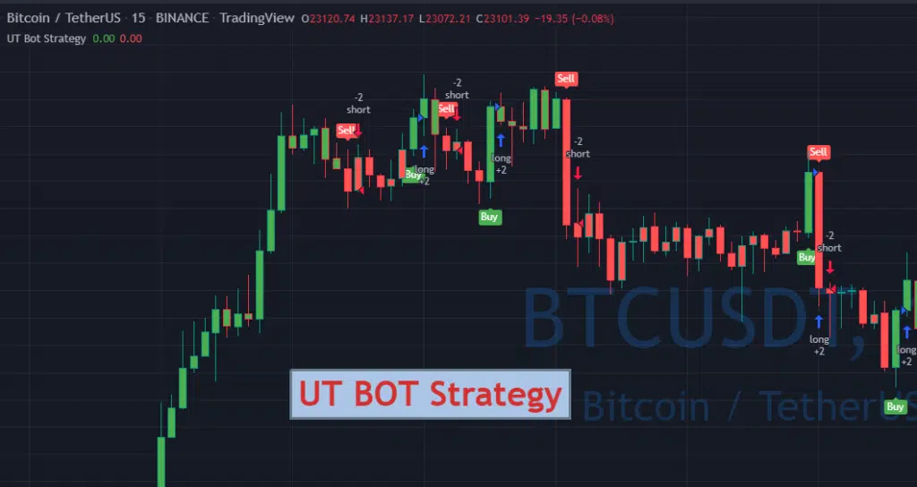
UT Bot Strategy is one of the most popular scripts I published on TradingView. I was asked many time if I have a version of this strategy in Python. Recently I started using vectorbt and I decided finally to implement this strategy in Python.
First let’s import all the libraries we’ll use in this code:
import vectorbt as vbt
import pandas as pd
import numpy as np
import talib
import datetime as dt

URL = 'https://api.binance.com/api/v3/klines'

intervals_to_secs = {
    '1m':60,
    '3m':180,
    '5m':300,
    '15m':900,
    '30m':1800,
    '1h':3600,
    '2h':7200,
    '4h':14400,
    '6h':21600,
    '8h':28800,
    '12h':43200,
    '1d':86400,
    '3d':259200,
    '1w':604800,
    '1M':2592000
}

def download_kline_data(start: dt.datetime, end:dt.datetime ,ticker:str, interval:str)-> pd.DataFrame:
    start = int(start.timestamp()*1000)
    end = int(end.timestamp()*1000)
    full_data = pd.DataFrame()

    while start < end:
        par = {'symbol': ticker, 'interval': interval, 'startTime': str(start), 'endTime': str(end), 'limit':1000}
        data = pd.DataFrame(json.loads(requests.get(URL, params= par).text))

        data.index = [dt.datetime.fromtimestamp(x/1000.0) for x in data.iloc[:,0]]
        data=data.astype(float)
        full_data = pd.concat([full_data,data])

        start+=intervals_to_secs[interval]*1000*1000

    full_data.columns = ['Datetime', 'Open', 'High', 'Low', 'Close', 'Volume','Close_time', 'Qav', 'Num_trades','Taker_base_vol', 'Taker_quote_vol', 'Ignore']

    return full_data
I’m importing vectorbt, pandas and numpy for some custom computations, binance api to get the candles for the backtest and talib for access to technical indicators in Python.
Next let’s define the parameters I want to use for my backtest. If you want to change any parameters for your backtest change them here:
# UT Bot Parameters
SENSITIVITY = 1
ATR_PERIOD = 10

# Ticker and timeframe
TICKER = "BTCUSDT"
INTERVAL = "1d"

# Backtest start/end date
START = dt.datetime(2017,8,17)
END   = dt.datetime.now()
Next let’s import data from Binance, with library I imported you can do it with 1 line of code:
# Get data from Binance
pd_data = download_kline_data(START, END, TICKER, INTERVAL)
Next I’ll compute ATR and NLoss variables. I’m using ATR function from TA lib to compute average true range, there are many other useful technical indicators available in this lib. Also I’ll delete all NAs to have a clean dataset.
# Compute ATR And nLoss variable
pd_data["xATR"] = talib.ATR(pd_data["High"], pd_data["Low"], pd_data["Close"], timeperiod=ATR_PERIOD)
pd_data["nLoss"] = SENSITIVITY * pd_data["xATR"]

#Drop all rows that have nan, X first depending on the ATR preiod for the moving average
pd_data = pd_data.dropna()
pd_data = pd_data.reset_index()
Next here is a function and a loop I’m using to compute ATRTrailingStop variable. It’s not the most efficient way to do that, but it 1 to 1 replicated logic from TradingView. I’ll take a look later how it can be computed without the loop.
# Function to compute ATRTrailingStop
def xATRTrailingStop_func(close, prev_close, prev_atr, nloss):
    if close > prev_atr and prev_close > prev_atr:
        return max(prev_atr, close - nloss)
    elif close < prev_atr and prev_close < prev_atr:
        return min(prev_atr, close + nloss)
    elif close > prev_atr:
        return close - nloss
    else:
        return close + nloss

# Filling ATRTrailingStop Variable
pd_data["ATRTrailingStop"] = [0.0] + [np.nan for i in range(len(pd_data) - 1)]

for i in range(1, len(pd_data)):
    pd_data.loc[i, "ATRTrailingStop"] = xATRTrailingStop_func(
        pd_data.loc[i, "Close"],
        pd_data.loc[i - 1, "Close"],
        pd_data.loc[i - 1, "ATRTrailingStop"],
        pd_data.loc[i, "nLoss"],
    )
In the following code I’ll compute “Buy” and “Sell” signals for my UT BOT Strategy:
# Calculating signals
ema = vbt.MA.run(pd_data["Close"], 1, short_name='EMA', ewm=True)

pd_data["Above"] = ema.ma_crossed_above(pd_data["ATRTrailingStop"])
pd_data["Below"] = ema.ma_crossed_below(pd_data["ATRTrailingStop"])

pd_data["Buy"] = (pd_data["Close"] > pd_data["ATRTrailingStop"]) & (pd_data["Above"]==True)
pd_data["Sell"] = (pd_data["Close"] < pd_data["ATRTrailingStop"]) & (pd_data["Below"]==True)
Next we’re ready to run the strategy itself:
# Run the strategy
pf = vbt.Portfolio.from_signals(
    pd_data["Close"],
    entries=pd_data["Buy"],
    short_entries=pd_data["Sell"],
    upon_opposite_entry='ReverseReduce',
    freq = "d"
)
To check the stats we can use stats() method:
pf.stats()
These will output us following stats for BTCUSDT 1d timeframe:
Start                                                  0
End                                                 1808
Period                                1809 days 00:00:00
Start Value                                        100.0
End Value                                     311.947976
Total Return [%]                              211.947976
Benchmark Return [%]                           435.91175
Max Gross Exposure [%]                             100.0
Total Fees Paid                                      0.0
Max Drawdown [%]                               60.805122
Max Drawdown Duration                  774 days 00:00:00
Total Trades                                         198
Total Closed Trades                                  197
Total Open Trades                                      1
Open Trade PnL                                  1.963699
Win Rate [%]                                   35.532995
Best Trade [%]                                126.663976
Worst Trade [%]                               -21.189107
Avg Winning Trade [%]                          15.214053
Avg Losing Trade [%]                           -5.996914
Avg Winning Trade Duration    14 days 20:54:51.428571428
Avg Losing Trade Duration      5 days 21:21:15.590551181
Profit Factor                                   1.096022
Expectancy                                       1.06591
Sharpe Ratio                                    0.672734
Calmar Ratio                                    0.424353
Omega Ratio                                     1.108914
Sortino Ratio                                   1.055846
dtype: object
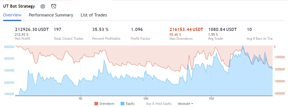
If we’re compare this metrics to TradingView’s metrics we’ll see that we’re matching exactly, this means that we implemented strategy correctly:
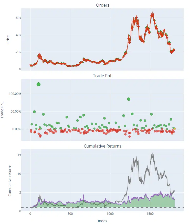
To plot the chart with P&L/signals and trades you can use following code:
# Show the chart
fig = pf.plot(subplots=['orders','trade_pnl','cum_returns'])
ema.ma.vbt.plot(fig=fig)
fig.show()
As you can see it’s not very complicated to code in Python even pretty advanced strategies like UT BOT. If you want me to implement other strategies in Python – let me know.
Follow me on TradingView and YouTube.


Awesome. I’d bet your profitability would be much better on an instrument with less abrupt price swings, like a stock or forex pair.
ERROR: Could not find a version that satisfies the requirement apis (from versions: none)
It’s a custom code to get data from Binance, here is this function:
URL = 'https://api.binance.com/api/v3/klines'
intervals_to_secs = {
'1m':60,
'3m':180,
'5m':300,
'15m':900,
'30m':1800,
'1h':3600,
'2h':7200,
'4h':14400,
'6h':21600,
'8h':28800,
'12h':43200,
'1d':86400,
'3d':259200,
'1w':604800,
'1M':2592000
}
def download_kline_data(start: dt.datetime, end:dt.datetime ,ticker:str, interval:str)-> pd.DataFrame:
start = int(start.timestamp()*1000)
end = int(end.timestamp()*1000)
full_data = pd.DataFrame()
while start < end: par = {'symbol': ticker, 'interval': interval, 'startTime': str(start), 'endTime': str(end), 'limit':1000} data = pd.DataFrame(json.loads(requests.get(URL, params= par).text)) data.index = [dt.datetime.fromtimestamp(x/1000.0) for x in data.iloc[:,0]] data=data.astype(float) full_data = pd.concat([full_data,data]) start+=intervals_to_secs[interval]*1000*1000 full_data.columns = ['Datetime', 'Open', 'High', 'Low', 'Close', 'Volume','Close_time', 'Qav', 'Num_trades','Taker_base_vol', 'Taker_quote_vol', 'Ignore'] return full_data
TA-Lib library not availble
Hi John,
You can install it in python: https://pypi.org/project/TA-Lib/
So.. one question, I’m trying to implement it not as a backtest, but live. I just cannot find the take-profit and stoploss in the code, only the ATRtrailingstop which is used to indicate when/whether to buy and sell.
When the buy/sell signal is produced, how would you determine the SL/TP?
Thanks in advance!
Joy
Check SL/PT examples here: https://quantnomad.com/using-sl-and-pt-in-backtesting-in-python-with-vectrobt/
Thank you, I got it. After executing your code, whole copy paste directly the output is not same or wrong.
tart 0
End 2403
Period 2404 days 00:00:00
Start Value 100.0
End Value -1817.297673
Total Return [%] -1917.297673
Benchmark Return [%] 1518.093694
Max Gross Exposure [%] 100.0
Total Fees Paid 0.0
Max Drawdown [%] 674.045678
Max Drawdown Duration 2301 days 00:00:00
Total Trades 31
Total Closed Trades 30
Total Open Trades 1
Open Trade PnL -2036.013137
Win Rate [%] 43.333333
Best Trade [%] 126.663976
Worst Trade [%] -20.708764
Avg Winning Trade [%] 22.977098
Avg Losing Trade [%] -8.584429
Avg Winning Trade Duration 14 days 14:46:09.230769230
Avg Losing Trade Duration 5 days 08:28:14.117647058
Profit Factor 1.363926
Expectancy 3.957182
Sharpe Ratio -0.513601
Calmar Ratio NaN
Omega Ratio 0.632677
Sortino Ratio -0.527403
dtype: object
Make sure you have the same data
The data is same, copy paste every thing.
Do you think is there any mistake in my program?
import vectorbt as vbt
import pandas as pd
import numpy as np
import talib
import datetime as dt
import requests
import json
import binance
URL = ‘https://api.binance.com/api/v3/klines’
intervals_to_secs = {
‘1m’: 60,
‘3m’: 180,
‘5m’: 300,
’15m’: 900,
’30m’: 1800,
‘1h’: 3600,
‘2h’: 7200,
‘4h’: 14400,
‘6h’: 21600,
‘8h’: 28800,
’12h’: 43200,
‘1d’: 86400,
‘3d’: 259200,
‘1w’: 604800,
‘1M’: 2592000
}
def download_kline_data(start: dt.datetime, end: dt.datetime, ticker: str, interval: str) -> pd.DataFrame:
start = int(start.timestamp() * 1000)
end = int(end.timestamp() * 1000)
full_data = pd.DataFrame()
while start prev_atr and prev_close > prev_atr:
return max(prev_atr, close – nloss)
elif close < prev_atr and prev_close prev_atr:
return close – nloss
else:
return close + nloss
# Filling ATRTrailingStop Variable
pd_data[“ATRTrailingStop”] = [0.0] + [np.nan for i in range(len(pd_data) – 1)]
for i in range(1, len(pd_data)):
pd_data.loc[i, “ATRTrailingStop”] = xATRTrailingStop_func(
pd_data.loc[i, “Close”],
pd_data.loc[i – 1, “Close”],
pd_data.loc[i – 1, “ATRTrailingStop”],
pd_data.loc[i, “nLoss”],
)
# Calculating signals
ema = vbt.MA.run(pd_data[“Close”], 1, short_name=’EMA’, ewm=True)
pd_data[“Above”] = ema.ma_crossed_above(pd_data[“ATRTrailingStop”])
pd_data[“Below”] = ema.ma_crossed_below(pd_data[“ATRTrailingStop”])
pd_data[“Buy”] = (pd_data[“Close”] > pd_data[“ATRTrailingStop”]) & pd_data[“Above”]
pd_data[“Sell”] = (pd_data[“Close”] < pd_data["ATRTrailingStop"]) & pd_data["Below"]
# Run the strategy
pf = vbt.Portfolio.from_signals(
pd_data["Close"],
entries=pd_data["Buy"],
short_entries=pd_data["Sell"],
upon_opposite_entry='ReverseReduce',
freq="d"
)
# print(pf.stats())
pf.stats()
# Show the chart
fig = pf.plot(subplots=['orders', 'trade_pnl', 'cum_returns'])
ema.ma.vbt.plot(fig=fig)
fig.show()
Awesome . Were you able to find a way to calculate the ATRTrailingStop variables without using the loop?
Hi Federico,
I’m not sure it’s possible to do that with vector. It’s past dependant.
What is the mathematical algorithm that vectorbt uses to calculate the signals Above & Below?
# Calculating signals
ema = vbt.MA.run(pd_data[“Close”], 1, short_name=’EMA’, ewm=True)
pd_data[“Above”] = ema.ma_crossed_above(pd_data[“ATRTrailingStop”])
pd_data[“Below”] = ema.ma_crossed_below(pd_data[“ATRTrailingStop”])
Thank you in advance for your response!
Well, I think it’s simply if first value for previous bar was below the second value, but now it’s above.