
vectorbt is the new Python Backtesting framework I’m using these days. I really like it so I decided to share an example of the simplest strategy built in the vecotrbt from scratch, so you can understand why I like it. This library is developed mostly in Pandas and Numpy so it should be really fast as well.
Let’s create a simple long only MA strategy. We’ll enter long when fast moving average cross over slow moving average and will close our position on the opposite cross.
Let’s start with importing the library:
import vectorbt as vbt
Next, I’ll download data from Yahoo Finance. There are many more other options, but for simplicity I’ll use build-in options for Yahoo finance:
data = vbt.YFData.download(
   'AAPL',
    interval = '1d'
)
This code will download daily OHLC data Apple stock for the entire history. In this backtest I’ll use only close data so I’ll create another variable with only close:
data_close = data.get('Close')
Next, let’s compute the moving averages we need for our signals. For that we can use build-in functions for moving average computations:
ma_fast = vbt.MA.run(data_close, 10)
ma_slow = vbt.MA.run(data_close, 50)
After MAs are computed we can create calculate our signals. Again I’ll use build-in functions for MA crosses:
entries = ma_fast.ma_crossed_above(ma_slow)
exits   = ma_fast.ma_crossed_below(ma_slow)
Now we have everything to run our backtest, in our case I’ll use “from_signal” function from vectorbt:
res = vbt.Portfolio.from_signals(
   data_close,
   entries = entries,
    exits = exits,
    freq = 'd'
)
So now our backtest is computed, so let’s check performance and other metrics of our strategy. To get basic metrics you can use stats() method of your backtesting results object:
res.stats()
This will output the following metrics:
Start                          1980-12-12 00:00:00+00:00
End                            2022-08-05 00:00:00+00:00
Period                               10501 days 00:00:00
Start Value                                        100.0
End Value                                  210757.880978
Total Return [%]                           210657.880978
Benchmark Return [%]                       165184.748186
Max Gross Exposure [%]                             100.0
Total Fees Paid                                      0.0
Max Drawdown [%]                               72.076296
Max Drawdown Duration                 1512 days 00:00:00
Total Trades                                         128
Total Closed Trades                                  127
Total Open Trades                                      1
Open Trade PnL                              19614.191557
Win Rate [%]                                   48.031496
Best Trade [%]                                115.002703
Worst Trade [%]                               -55.651257
Avg Winning Trade [%]                          25.743169
Avg Losing Trade [%]                           -7.004448
Avg Winning Trade Duration    79 days 19:16:43.278688524
Avg Losing Trade Duration     21 days 09:05:27.272727272
Profit Factor                                   3.360768
Expectancy                                   1504.281019
Sharpe Ratio                                    0.883608
Calmar Ratio                                    0.422827
Omega Ratio                                     1.191955
Sortino Ratio                                   1.300257
dtype: object
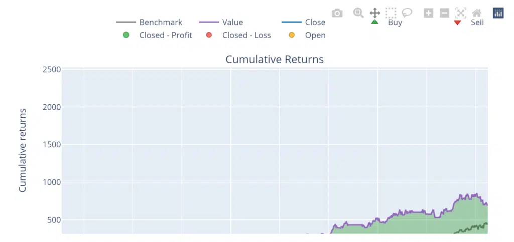
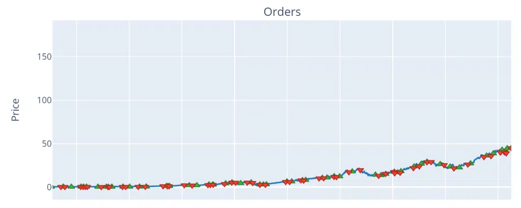
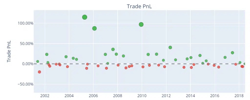
It’s quite easy to plot nice charts with metrics and signals. For that, you can use the plot() method specifying what plots you want to compute over the backtesting results.
fig = res.plot(subplots = ['cum_returns', 'orders', 'trade_pnl'])
fig.show()
This will output you 3 plots. All these plots will be dynamic plots built with plotly, so you can zoom on it, explore details, etc.
If you want a bit more details about your strategy you can get a detailed summary of your trades:
res.positions.records_readable
This code will output you a nice pandas data frame with some metrics for all your trades:

So that’s it, As you can see it’s a really nice library that will allow you to code backtests and explore your strategies just in a few lines of code. I think I’ll create more content about it, so let me know what you want to know about it.
Here is full code used in this article:
import vectorbt as vbt

data = vbt.YFData.download(
   'AAPL',
    interval = '1d'
)

data_close = data.get('Close')

ma_fast = vbt.MA.run(data_close, 10)
ma_slow = vbt.MA.run(data_close, 50)

entries = ma_fast.ma_crossed_above(ma_slow)
exits   = ma_fast.ma_crossed_below(ma_slow)

res = vbt.Portfolio.from_signals(
   data_close,
   entries = entries,
    exits = exits,
    freq = 'd'
)

res.stats()

fig = res.plot(subplots = ['cum_returns', 'orders', 'trade_pnl'])
fig.show()

res.positions.records_readable
Follow me on TradingView and YouTube.