Running Grid Optimization for Backtests in Python using vectorbt

After running backtests, many quants want to know the best parameters for their strategies. For that, you can run one of the optimization algorithms that will find the best combination of parameters to give you the best metrics you want to optimize. It’s a pretty helpful feature, and many quants use it. However, you must use it carefully because it’s pretty easy to overfit your strategy.

In this article, I’ll show you how to code and run grid optimization in Python. It’s the easiest way to perform optimization. In short, we’ll create a grid of different parameters we want to try and then run a backtest for all of them. As a result, we’ll see the performance of all of them and can select the best one to trade. In the article, I’m using vector, my favorite framework for backtesting. You’ll see it’s really easy to run grid optimization using vectorbt.

To get the data, I’m using Polygon API, one of the best data APIs for market data. You can use the “QUANTNOMAD10” code to get 10% discount for any of their subscriptions.

Let’s start by loading the libraries needed in our code. I’m using all the essential libraries I always use here in my analysis.

import vectorbt as vbt
import talib as ta
import numpy as np
import pandas as pd
from polygon import RESTClient

pd.set_option('display.max_rows', 50)

Loading data

Next, I’ll load the data. I’ll load BTCUSDT 1-minute bars for the last two weeks from Polygon.io. In total, it will be around 20k rows. Polygon allows you to load up to 50k minute bars in 1 go.

client = RESTClient(api_key="YOUR_POLYGON_API_KEY")

btc = pd.DataFrame(
    client.get_aggs(
        ticker="X:BTCUSD", 
        multiplier=1, 
        timespan="minute", 
        from_="2023-03-12", 
        to="2023-03-26", 
        limit = 20000)
)

Results returned by Polygon are already pretty clean and don’t require any additional changes before the analysis:

Defining Strategy

Now let’s define the strategy we want to optimize. I’ll create a function for a very basic RSI strategy:

• When RSI crosses over oversold level -> Long Signal
• When RSI crossed under overbought level -> Short Signal.

Here is the function that computes everything and outputs long and short signals. You can see that I pass all the parameters to the function. This way, we’ll be able to run grid optimization on it.

def rsi_signals_indicator(close, length = 14, ob_level = 70, os_level=30):
    rsi = ta.RSI(close, length)

    long_signals  = np.where(np.logical_and(pd.Series(rsi).shift(1) < os_level, rsi >= os_level), 1, 0)
    short_signals = np.where(np.logical_and(pd.Series(rsi).shift(1) > ob_level, rsi <= ob_level), 1, 0)

    return long_signals,short_signals

The output of this function will be only two arrays with zeroes and ones representing short and long signals:

[l,s] = rsi_signals_indicator(btc['close'], length = 14, ob_level = 70, os_level=30)
l

array([0, 0, 0, ..., 0, 0, 0])

Now we can define our RSI indicator the vectorbt way. We’ll use an IndicatorFactory method to do that. We’ll pass to its name, parameters, and function itself:

RSI_indicator = vbt.IndicatorFactory(
    class_name="RSI Indicator",
    short_name="RSI Ind",
    input_names=["close"],
    param_names=["length","ob_level","os_level"],
    output_names=["long_signals","short_signals"]
).from_apply_func(
    rsi_signals_indicator,
    length   = 14,
    ob_level = 70,
    os_level = 30,
    to_2d = False
)

Defining parameters grid

Now we need to define what parameters combination we want to test. Here is an example of arrays I defined for that. For every one of the parameters, I defined ten values I want vectorbt to try:

length_arr   = np.arange(10,20)
os_level_arr = np.arange(20,30)
ob_level_arr = np.arange(70,80)

To initialize the grid, we have to run out Indicator with these parameters arrays passed to it following way:

ind_grid = RSI_indicator.run(
    btc.close, 
    length    = length_arr,
    ob_level  = ob_level_arr, 
    os_level  = os_level_arr, 
    param_product = True 
)

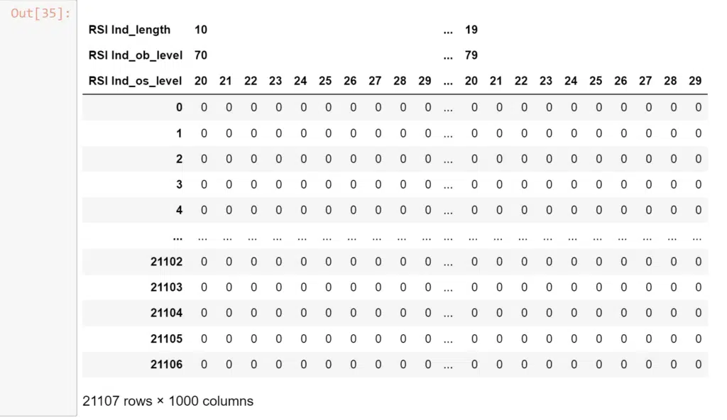
This will output us an object containing Long and Short signals vectors computed for all possible combinations of parameters I send to it. For example let’s check long signals:

ind_grid.long_signals

You can see that it outputs a huge matrix with 20M+ elements. It stores full long/short vectors for every parameter combination, so you have to be careful with the size of the optimization you’re running, so it fits the memory of your PC.

Running Backtest

Now it’s all ready for the backtest calculations. To do that, we can pass our gird vector to the from_signal method of vectorbt:

# Only long
pf_long = vbt.Portfolio.from_signals(
    btc.close,
    entries = ind_grid.long_signals,
    exits   = ind_grid.short_signals,
)

What I like about vectorbt is that it’s pretty fast. This pretty big grid optimization will take only a few seconds to run. You can export parameters from the backtesting with a stats method. Let’s export essential metrics for our grid optimization.

stats_long = pf_long.stats([
    'total_return',
    'total_trades',
    'win_rate',
    'expectancy', 
    'profit_factor'
], agg_func=None)

stats_long

This will output us a nice data frame with a raw for every parameter combination:

To find the best parameters from this data frame, you can sort it by one of the metrics like this:

stats_long.sort_values("Profit Factor", ascending=False)

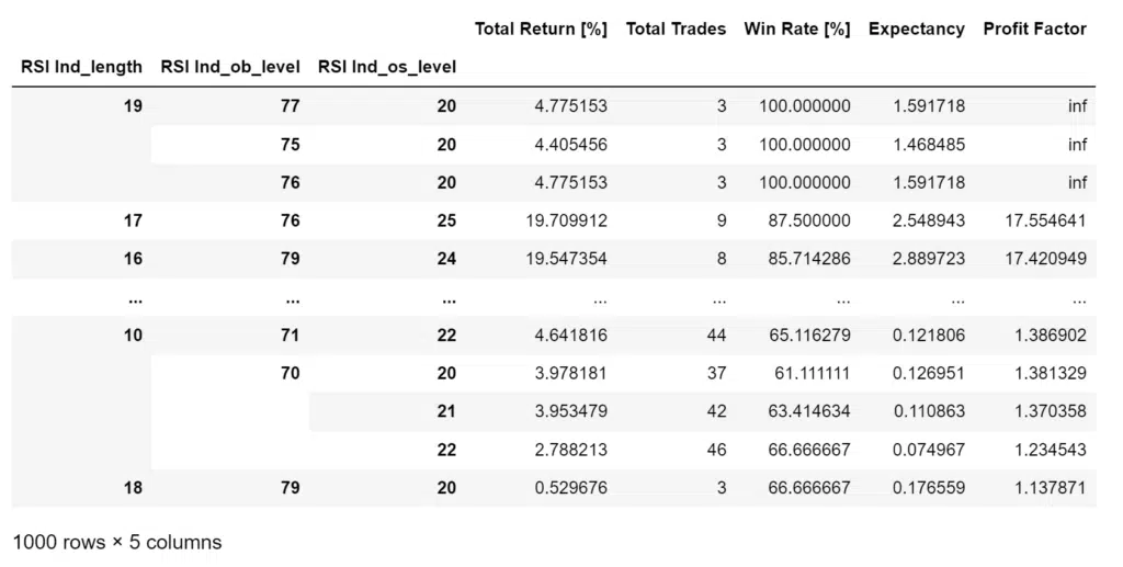
Be careful with this approach. It’s pretty easy to overfit a strategy using optimization. Try to select parameters with more trades and avoid local maximums – parameter combinations with a much worse performance with parameters slightly different.

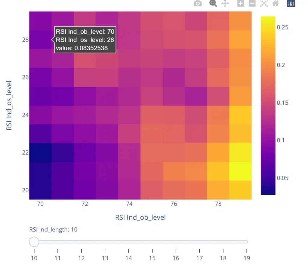
Another practical way to explore gird optimization results is to plot a heatmap using the vbt.heatmap method. This will plot us a 2d heatmap with a selected performance coded as colors. Also, you can provide a 3rd parameter to be a slider to explore your grid in 3d.

long_returns = pf_long.total_return()

fig = long_returns.vbt.heatmap(
    x_level = "RSI Ind_ob_level",
    y_level = "RSI Ind_os_level",
    slider_level = "RSI Ind_length"
)

fig.show()

Disclaimer
Please remember that past performance may not indicate future results.
Due to various factors, including changing market conditions, the strategy may no longer perform as well as in historical backtesting.
This post and the script don’t provide any financial advice.

Follow me on TradingView and YouTube.